Plotting Points Method
- Find ordered pair solutions
- Choose values for one variable
- Find the value for the other variable
- Plot the ordered pair solutions
- Draw the line or curve that connects the ordered pairs
Example: Graph  by the plotting points method.
1. Find ordered pair solutions. We can organize this information in a table.
- Choose values for one variable
When the equation is written in “y=” format it is easier to choose values for x and then find the y’s. For this table I will choose multiples of the denominator so that my ordered pairs are all integers.
| x | y |
|---|---|
| 3(-2)=-6 | |
| 3(-1)=-3 | |
| 3(0)=0 | |
| 3(1)=3 | |
| 3(2)=6 |
- Find the values for the other variable
To find the y’s substitute the value of x into the equation and simplify to find y.
| x | y | y | y |
|---|---|---|---|
| -6 | -1/3(-6)+2= | 2+2= | 4 |
| -3 | -1/3(-3)+2= | 1+2= | 3 |
| 0 | -1/3(0)+2= | 0+2= | 2 |
| 3 | -1/3(3)+2= | -1+2= | 1 |
| 6 | -1/3(6)+2= | -2+2= | 0 |
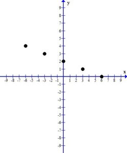
2. Plot the ordered pair solutions
Using the table above we have 5 ordered pairs , (-3, 3), (0, 2), (3, 1), (6, 0)")
Plot the ordered pairs using the rectangular coordinate system.
3. Draw the line or curve that connects the ordered pairs.
When you look at the plotted ordered pairs you should see a pattern the that points make. In this case, the points form a straight line.
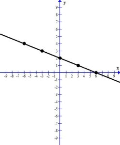
The line represents all of the ordered pairs that are solutions to the equation  .
.
Here is a youtube video with a similar example.
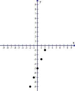
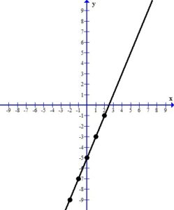
 by the plotting points method.
, (-1, -7), (0, -5), (1, -3), (2, -1)")
}=L") .
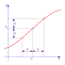
. > 0 there exist
  >0 such that
 <
< -L}{|}") <
<  .
.
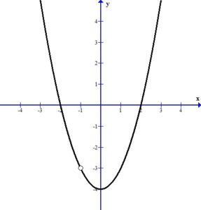
 = {x^3+x^2-4x-4}/{x+1}")
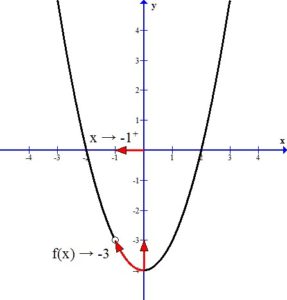
 right -3") as
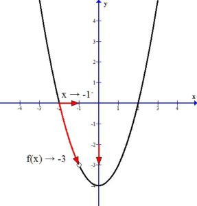
as  from the left would be written.
}=-3")
}=-3")
}=-3")
-4(x+1)}/{x+1} }")
(x+1)}/{x+1}}")