All posts by admin

Graphing a Linear Equation by Plotting Points (m is a fraction)

Plotting Points Method

  1. Find ordered pair solutions
    • Choose values for one variable
    • Find the value for the other variable
  2. Plot the ordered pair solutions
  3. Draw the line or curve that connects the ordered pairs

Example: Graph  y= -{1}/{3}x+2 by the plotting points method.

1. Find ordered pair solutions.  We can organize this information in a table.

  • Choose values for one variable

When the equation is written in “y=” format it is easier to choose values for x and then find the y’s.  For this table I will choose multiples of the denominator so that my ordered pairs are all integers.

xy
3(-2)=-6
3(-1)=-3
3(0)=0
3(1)=3
3(2)=6
  • Find the values for the other variable

To find the y’s substitute the value of x into the equation and simplify to find y.

xyyy
-6-1/3(-6)+2=2+2=4
-3-1/3(-3)+2=1+2=3
0-1/3(0)+2=0+2=2
3-1/3(3)+2=-1+2=1
6-1/3(6)+2=-2+2=0

2.  Plot the ordered pair solutions

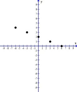
Using the table above we have 5 ordered pairs (-6, 4), (-3, 3), (0, 2), (3, 1), (6, 0)

Plot the ordered pairs using the rectangular coordinate system.
3.  Draw the line or curve that connects the ordered pairs.

When you look at the plotted ordered pairs you should see a pattern the that points make.  In this case, the points form a straight line.
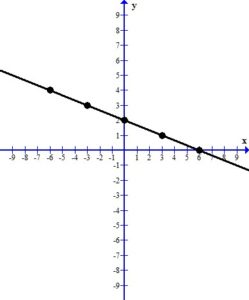
The line represents all of the ordered pairs that are solutions to the equation y= - {1} / {3}x+2.

Here is a youtube video with a similar example.

Graphing a Linear Equation by Plotting Points (m is an integer)

Plotting Points Method

  1. Find ordered pair solutions
    • Choose values for one variable
    • Find the value for the other variable
  2. Plot the ordered pair solutions
  3. Draw the line or curve that connects the ordered pairs


Example: Graph  y= 2x-5 by the plotting points method.

1. Find ordered pair solutions.  We can organize this information in a table.

  • Choose values for one variable

When the equation is written in “y=” format it is easier to choose values for x and then find the y’s.  Although you are allowed to choose any x values, for this table I have used a standard set of x’s so that we have a variety.  Some negatives, some positives and zeros.

xy
-2
-1
0
1
2
  • Find the values for the other variable

To find the y’s substitute the value of x into the equation and simplify to find y.

xy
-22(-2)-5=-4-5=-9
-12(-1)-5=-2-5=-7
02(0)-5=0-5=-5
12(1)-5=2-5=-3
22(2)-5=4-5=-1

2.  Plot the ordered pair solutions

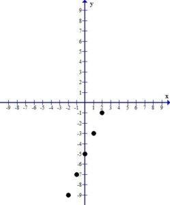
Using the table above we have 5 ordered pairs (-2, -9), (-1, -7), (0, -5), (1, -3), (2, -1)

Plot the ordered pairs using the rectangular coordinate system.

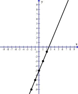
3.  Draw the line or curve that connects the ordered pairs.

When you look at the plotted ordered pairs you should see a pattern the that points make.  In this case, the points form a straight line.

The line represents all of the ordered pairs that are solutions to the equation y= 2x-5.

Here is a youtube video with a similar example


Dividing Out Technique

The first technique we discussed for finding a limit analytically is direct substitution. That strategy doesn’t work when we get an indeterminate form from the substitution such as 0/0.

One strategy to handle this form is the dividing out technique. This is where you factor both the numerator and denominator and cancel any common factor.

Here are some video examples.

This example has a quadratic to factor.


The first example in this video uses a special factoring technique called difference of squares. The second example in this video avoids factoring by using synthetic division to divide out.

The second example in this video matches the 2nd example in the video above but using the special factoring technique of difference of cubes instead of using synthetic division.


This video has an example that reviews factoring trinomials with a not equal 1.


Formal Definition of a Limit

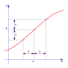
Let f be a function defined on an open interval containing c (except possibly c), and let L be a real number. The statement

lim{x right c}{f(x)}=L.

means that for each {epsilon} > 0 there exist delta>0 such that

0< delim{|}{x-c}{|} < delta then delim{|}{f(x)-L}{|} < epsilon .

Límite_01.svg

Here is a video that demonstrates how to prove the limit is L using the delta-epsilon definition.

Limit at a Hole

The function f below is undefined for x=-1. Using a table, analyze what is happening to f(x) as x approaches -1.

f(x) = {x^3+x^2-4x-4}/{x+1}

Filling out this table will help us decide what is happening to f(x) as x is getting closer to -1 from the left. (x’s that are smaller then -1)

x-1.1-1.01-1.001-1.0001-1
f(x)?

Filling out this table will help us decide what is happening to f(x) as x is getting closer to -1 from the right. (x’s that are larger then -1)

x-.9-.99-.999-.9999-1
f(x)?

Here is a video that will help you use the features in your calculator to fill in the values of the table:

x-1.1-1.01-1.001-1.0001-1
f(x)-2.79-2.9799-2.998-2.9998?

As you can see from the table, f(x) approaches -3 as x approaches -1 from the left. Symbolically f(x) right -3as x right -1 from the left would be written.
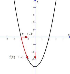
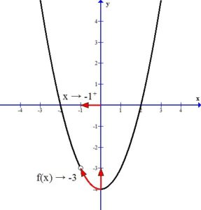
lim{x right -1^{-}}{f(x)}=-3

x-.9-.99-.999-.9999-1
f(x)-3.19-3.0199-3.002-3.0002?

As you can see from the table, f(x) approaches -3 as x approaches -1 from the right. Symbolically f(x) right -3as x right -1 from the right would be written.

lim{x right -1^{+}}{f(x)}=-3

These are called one sided limits.

Informal Definition of a Limit: If f(x) becomes arbitrarily close to a single number L as x approaches c from either side, then the limit of f(x) , as x approaches c is L.

In general: lim{x right c}{f(x)}=L

In our example, f(x) becomes arbitrarily close to -3 as x approaches -1 from the left and right.

lim{x right -1}{f(x)}=-3

Limit at a Hole

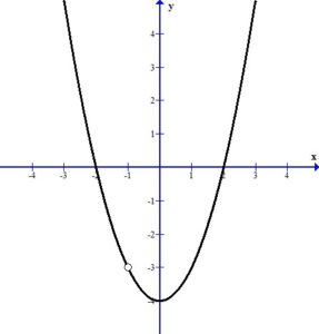
Use the graph, estimate the limit as x approaches -1.

f(x) = {x^3+x^2-4x-4}/{x+1}

The function f above is undefined for x=-1. By simplifying f(x) we find a function whose graph agrees with f(x) at every point except -1.

f(x) = {x^3+x^2-4x-4}/{x+1}

{= {x^2(x+1)-4(x+1)}/{x+1} }

{={(x^2-4)(x+1)}/{x+1}}

{=x^2-4}

Since f(x) is undefined for x=-1 and we were able to cancel a common factor of x+1 from the numerator and denominator there is a hole in the graph of f(x) at x=-1

Graph with hole


For f(x) to have a limit as x approaches -1 the one-sided limits must agree.

From the right:

Graph with hole right limit

lim{x right -1^{+}}{f(x)}=-3

From the left:

Graph with hole left limit

lim{x right -1^{-}}{f(x)}=-3

Since the one-sided limits agree, the limit exists.

lim{x right -1}{f(x)}=-3


Here are some practice problems.

MAC2311 Limits Graphically